, (1)
, (1)
WSRC-TR-2000-00132
A Spreadsheet Program for Steady-State Temperature Fields
Gregory J. Hutchens and Narendra K. Gupta
Westinghouse Savannah River Company
Savannah River Site
Aiken, SC 29808
This report was prepared as an account of work sponsored by an agency of the United States Government. Neither the United States Government nor any agency thereof, nor any of their employees, makes any warranty, express or implied, or assumes any legal liability or responsibility for the accuracy, completeness, or usefulness of any information, apparatus, product or process disclosed, or represents that its use would not infringe privately owned rights. Reference herein to any specific commercial product, process or service by trade name, trademark, manufacturer, or otherwise does not necessarily constitute or imply its endorsement, recommendation, or favoring by the United States Government or any agency thereof. The views and opinions of authors expressed herein do not necessarily state or reflect those of the United States Government or any agency thereof.
This report has been reproduced directly from the best available copy.
Available for sale to the public, in paper, from: U.S. Department of Commerce, National Technical Information Service, 5285 Port Royal Road, Springfield, VA 22161, phone: (800) 553-6847, fax: (703) 605-6900, email: orders@ntis.fedworld.gov online ordering: http://www.ntis.gov/support/ordering.htm
Available electronically at http://www.osti.gov/bridge/
Available for a processing fee to U.S. Department
of Energy and its contractors, in paper, from: U.S. Department of Energy, Office
of Scientific and Technical Information, P.O. Box 62, Oak Ridge, TN 37831-0062,
phone: (865 ) 576-8401, fax: (865) 576-5728, email: reports@adonis.osti.gov
Abstract
A spreadsheet macro program is developed in EXCEL using Visual Basic for Applications (VBA) to analyze two-dimensional heat transfer. A description of the physical system analyzed is given along with the model equations and numerical methods used. The macro program is described and results of the analysis presented.
Introduction
In the last decade, spreadsheet programs such as EXCEL have advanced far beyond their original financial and office environment applications. Today, spreadsheets are a common tool used in engineering analyses, including the numerical solution of engineering boundary value problems.2, 5 The objective here is to use an EXCEL spreadsheet to analyze an engineering problem of practical interest, namely, estimate the two-dimensional steady-sate temperature distribution in a concrete wall subject to thermal radiation on one of its boundaries. The analysis will include the numerical solution of the nonlinear heat conduction problem associated with determining the temperature distribution in the wall. Then, output from the numerical solution will be used to construct surface plots showing the spatial distribution of the temperature.
First, background information will be provided where the physical configuration of the system being analyzed is described and the motivation for the analysis is given. Next, the basic energy balance is described which leads to the model equations giving the required steady-state heat conduction equation and boundary conditions. Then, the finite difference approximations of the model equations are derived and the program used to implement the solution algorithm is described. Finally, the results of the analysis are presented and discussed. Based on the results, conclusions are drawn and recommendations for further work are given.
Background
A bank of high-pressure steam lines passes through the north wall penetration of the Replacement High Level Waste Evaporator (RHLWE) at the Savannah River Site. The steam lines that pass through the wall penetration are not insulated. The steam lines rest on a W4X13 stainless steel I-Beam. This I-Beam rests on a stainless steel plate (part of the wall penetration) which is embedded in the concrete wall. There is concern that the high temperature (430 oF) steam pipes will heat the concrete around the penetration well above 200 oF and degrade its strength properties. However, if the depth of the temperature increase around the wall penetration is limited to a few inches, the loss of concrete strength can be treated as local and the wall structural integrity will not be adversely affected. This calculation determines the temperature field around the penetration and in the wall under steady-state conditions. The arrangement of the steam lines and the wall penetration is shown schematically in Fig. 1.
The concrete wall below the penetration is modeled as a two-dimensional slab. The wall is 35 feet high and 3.5 feet thick. Any cylindrical effects due to the steam pipe are neglected. Due to the size of the wall, corrections due to the effects of curvature will be small. Further, since the thermal radiation will be emitted in all directions from the cylindrical surface of the steam pipe, the concrete wall above the penetration will behave similarly. The only difference in the temperature profile in the concrete wall above the penetration will be due to a difference in the boundary conditions. Finally, it is assumed that the thermal radiation is emitted from a flat surface with normal incidence, that is, the effect of radiation view factors has been neglected. Including the radiation view factors will reduce the incident thermal radiation by correcting for the effects of cylindrical geometry and the opening into the evaporator cell. See Figure 2 for the coordinate directions along with the required boundary conditions.
Model Equations
Energy, in the form of heat, enters the surface of the concrete wall in the form of thermal radiation. This energy is then conducted throughout the wall and removed from the sides by free convection to the air at temperature, Tair, and to the evaporator cell floor at temperature, Tfloor. To provide orientation within the wall, take the surface of the wall at the penetration as x = 0 ft and measure x positive in the downward direction. Hence, the floor is at x = 35 ft. Likewise, take the vertical centerline of the wall as y = 0 ft. Then, the outer wall is at y = 1.75 ft.
For steady energy flow in the concrete wall, the energy balance reduces to the steady-state heat conduction equation without heat generation, namely,
, (1)
where T is the concrete temperature (in oF). The boundary conditions, which govern the energy flow into and out of the wall, are as follows. For thermal radiation at the wall penetration (x = 0)
 , (2)
, (2)
where k is the thermal conductivity of the concrete (in Btu/hr-ft-oF), s is the Stefan-Boltzmann constant (0.1714´ 10-8 Btu/hr-ft2- R4), a is the fraction of incident thermal radiation that is absorbed in the concrete (assumed to be 1), Ts is the temperature of the steam line (in oF), and the factor of 459.67 is required to convert the temperature from units of oF to R. For the base of the slab which is maintained at the constant temperature, Tfloor,
 , (3)
, (3)
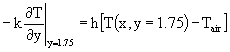
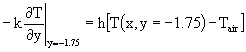
where Tfloor is the evaporator cell temperature (in oF, assumed constant). For free convection cooling along the vertical outer surfaces of the wall (y = ± 1.75 ft),
 , (4)
, (4)
 . (5)
. (5)
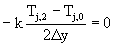
Note that since the same air temperature is used on both sides of the wall, the temperature distribution within the wall will be symmetric in y. Hence, Eq. (5) may be replaced by the "reflecting" boundary condition
 . (6)
. (6)
In Eq. (4), h is the free convection heat transfer coefficient for the vertical wall (in Btu/hr-ft2-oF), and Tair is the ambient air temperature (in oF, assumed constant).
Due to the nonlinear boundary condition, Eq. (2), the model problem is difficult to solve, even though the energy balance, Eq. (1), and the remaining boundary conditions are linear. An approximate analytical solution may be constructed by linearizing the radiation boundary condition namely,
 . (7)
. (7)
then, classical methods for solving linear partial differential equations, such as integral transforms, may be used to solve for the temperature distribution. On the other hand, the model problem, including the nonlinear boundary condition, is relatively straightforward to solve numerically.
Finite Difference Equations
To derive the finite difference form of the energy balance, Eq. (1), and boundary conditions, Eqs. (2)-(4) and (6), associate the index "j" with the x-coordinate and the index "k" with the y-coordinate so that the temperature, T(x, y), becomes Tj,k. Then, the energy balance and boundary conditions are averaged over a finite difference zone of "volume" D xD y (where it is assumed that D x and D y are constant but not necessarily equal). For example, the energy balance, Eq. (1), becomes
 . (8)
. (8)
Carrying through the integration gives the finite difference approximation for Eq. (1), namely,
 . (9)
. (9)
Likewise, the boundary conditions become,
 , (10)
 , (11)
 , (12)
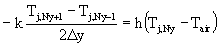 , (13)
where Nx and Ny are the maximum number of grid points in the x- and y-directions, respectively.
Eqs. (9) through (13) form a pentadiagonal system of algebraic equations. Due to the large number of zero elements in the system (that is, the system is sparse), direct methods of solution (e.g., Gaussian elimination) are both time consuming and inefficient. A straightforward alternative is iterative methods. Furthermore, since the radiation boundary condition, Eq. (10), is nonlinear, a particularly useful iterative method is Newton’s method.1 To apply Newton’s method to Eq. (9) through (13), make the substitution 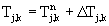 , where
  is known and D
Tj,k is a small correction. The resulting set of algebraic equations for D
Tj,k may be solved, for example, by Gauss-Seidel iteration. Note that by making this substitution analytically, the difficult and time-consuming task of numerically evaluating the partial derivatives of the Jacobian matrix required by Newton’s method is eliminated. This results in shorter execution time and increased precision of the results.
is known and D
Tj,k is a small correction. The resulting set of algebraic equations for D
Tj,k may be solved, for example, by Gauss-Seidel iteration. Note that by making this substitution analytically, the difficult and time-consuming task of numerically evaluating the partial derivatives of the Jacobian matrix required by Newton’s method is eliminated. This results in shorter execution time and increased precision of the results.
Program Description
A program to solve the above set of difference equations has been developed in EXCEL using Visual Basic for Applications (VBA).6 Prior to version 5, EXCEL used a macro language called XLM. With XLM it was possible to group together functions (XLM commands) to form rudimentary programs. These programs could then be used in various applications. However, beginning with version 5, EXCEL introduced VBA as the macro language that offers several advantages over XLM, including maintainability of the macro code.
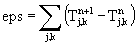
The VBA program takes as input the spatial step size in the x-direction, D x. This is entered in cell A1 of the EXCEL Worksheet. Other required data, such as the spatial step in the y-direction, D y, and other physical data (e.g., thermal conductivity) are, at present, declared constants in the VBA code. After reading D x the code calculates the maximum number of zones in the x- and y-directions, Nx and Ny, respectively, and initializes the boundary conditions. The code then enters the main iteration loop that terminates when the error, defined as the sum of the difference between iterates, eps, is less than 0.01. This is calculated as
 . (14)
Upon reaching the required convergence, the code prints the estimated error and number of iterations performed in cells B1 and B3. The code then prints the computed temperature distribution in the wall for all x-coordinates in columns C through N. The code may be executed from the EXCEL Tool Bar drop down menu (ToolsÞ Macros) or by placing a control button on the EXCEL Worksheet.
Data and Results
Physical data used to solve Eqs. (9) through (13) are as follows:
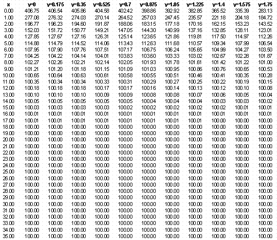
With the above data, Eqs. (9) through (13) are solved to determine the steady-state temperature in the concrete wall. Choosing Tair and Tfloor to be 100 oF will results in conservative estimates of the temperature distribution inside the concrete wall. In reality both Tair and Tfloor will be less than 100 oF resulting in a concrete temperature which is lower than that calculated. Furthermore, by choosing the other physical parameters (k, h, etc.) at the low end of their range will also provide conservatism in the temperature estimate. Hence, if the spatial temperature distribution does not exceed the limit imposed by the structural analysis, then the actual temperature in the concrete wall will not exceed the limit as well. Results are given in Table 1 for the model problem.
Fig. 3 shows a surface plot of the temperature distribution in the upper ten feet of the wall. Notice that from the surface of the wall (x = 0), the temperature relaxes to less than 200 oF approximately two feet into the slab. This is, obviously, due to the low thermal conductivity of the concrete in the wall. Indeed, the high temperature in the wall near the surface may be attributed to both the radiant heat flux entering the surface and the slow rate of heat removal due to conduction. For higher values of thermal conductivity the wall temperature near the surface is reduced but the depth of wall affected is increased. That is, the temperature is above 200 oF deeper in the wall, just as expected.
Fig. 4 shows a surface plot of the temperature distribution in the upper ten feet of the wall as a result of solving the linear model problem, Eq. (9) through (12) and the finite difference approximation of Eq. (7). Comparing Figs. 3 and 4 shows that the solution of the linear model problem exhibits the correct qualitative shape, relaxing from the peak temperature at the surface to less than 200 oF at approximately the same depth (less than 2 ft). In fact, in Fig. 4 it is seen that the principal difference between the linear and nonlinear model problems is that of magnitude. Due to the approximate treatment of the nonlinear boundary condition, Eq. (7), the linear problem underpredicts the temperature in the region of interest.
Fig. 5 shows a surface plot of the temperature difference between the linear and nonlinear model problems. As expected, as wall depth increases the temperature difference decreases. This is, again, due to the low thermal conductivity of the concrete in the wall which determines the length scale over which the temperature changes. Beyond a certain depth the effect of the boundary condition at the surface (x = 0) is negligible and the temperature difference vanishes. Finally, Fig. 6 shows a surface plot of the temperature distribution in the entire wall.
Conclusion
Using Visual Basic for Applications (VBA), a spreadsheet macro program has been developed in EXCEL to calculate two-dimensional steady-state temperatures. This macro program was then used to determine the temperature distribution in the wall at the Replacement High Level Waste Evaporator at the Savannah River Site. Due to a steam line penetration through the wall, the wall surface is subjected to thermal radiation, which imposes a nonlinear boundary condition.
For the conservative assumption that all incident thermal radiation is absorbed, as well as using conservative values for various physical parameters (e.g., thermal conductivity), it is seen that from the surface of the wall (x = 0), the temperature relaxes to less than 200 oF approximately two feet into the slab. In fact, for more realistic values of the wall surface absorptivity (a less than 1), both the wall surface temperature and relaxation depth are reduced.
Although this macro program was developed for a particular application, several straightforward modifications could significantly enhance its utility. Rather than including the physical data as declared constants in the body of the code, the data could be entered on the EXCEL Worksheet (along with D x) and read into the code. Or VBA visual programming tools could be used to create dialog boxes that prompt the user for input. In addition, several different boundary conditions could be included as a set of options for the user to select. The creation of data charts and plots could also be automated using VBA. Finally, the model problem could be extended to three-dimensions or transient analysis, although the transient analysis may require a different numerical technique, for efficiency.
Acknowledgements
This work was performed under the auspices of the U. S. Department of Energy under contract DE-AC09-96SR18500.
References
G. Golub and J. M. Ortega, Scientific Computing, An Introduction with Parallel Computing, (Academic Press: San Diego, CA, 1993).
Figure. 1. Schematic of concrete wall penetration
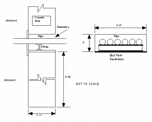
Figure. 2. Coordinate directions and boundary conditions
Figure 3. Temperature distribution for model problem
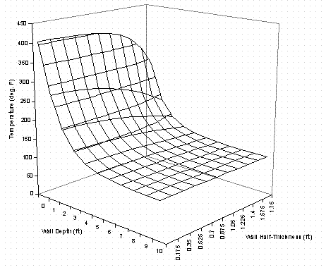
Figure 4. Temperature distribution for linear model problem
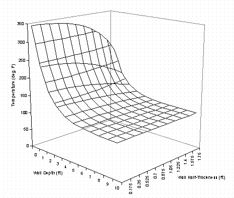
Figure 5. Temperature difference between linear and nonlinear model problems
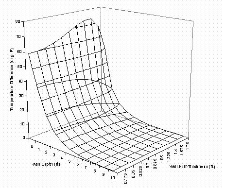
Figure 6. Temperature distribution in wall
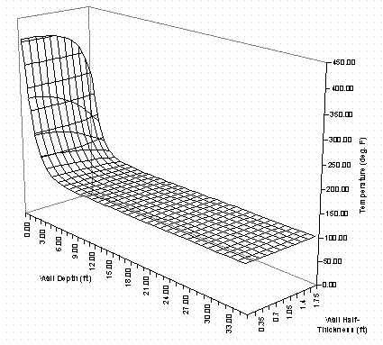
Table I. Results for model problem