WSRC-MS-2001-00145
Using Geoscience and Geostatistics to Optimize
Groundwater
Monitoring Networks at the Savannah River Site
R. C. Tuckfield, E. P. Shine, R. A. Hiergesell, M. E. Denham, and S. Reboul
Westinghouse Savannah River Company
Aiken, SC 29808
C. Beardsley
Bechtel Savannah River Inc.
Aiken, SC 29808
This report was prepared as an account of work sponsored by an agency of the United States Government. Neither the United States Government nor any agency thereof, nor any of their employees, makes any warranty, express or implied, or assumes any legal liability or responsibility for the accuracy, completeness, or usefulness of any information, apparatus, product or process disclosed, or represents that its use would not infringe privately owned rights. Reference herein to any specific commercial product, process or service by trade name, trademark, manufacturer, or otherwise does not necessarily constitute or imply its endorsement, recommendation, or favoring by the United States Government or any agency thereof. The views and opinions of authors expressed herein do not necessarily state or reflect those of the United States Government or any agency thereof.
This report has been reproduced directly from the best available copy.
Available for sale to the public, in paper, from: U.S. Department of Commerce, National Technical Information Service, 5285 Port Royal Road, Springfield, VA 22161, phone: (800) 553-6847, fax: (703) 605-6900, email: orders@ntis.fedworld.gov online ordering: http://www.ntis.gov/support/ordering.htm
Available electronically at http://www.osti.gov/bridge/
Available for a processing fee to U.S. Department of Energy and its contractors, in paper, from: U.S. Department of Energy, Office of Scientific and Technical Information, P.O. Box 62, Oak Ridge, TN 37831-0062, phone: (865 ) 576-8401, fax: (865) 576-5728, email: reports@adonis.osti.gov
Abstract
A team of scientists, engineers, and statisticians was assembled to review the operation efficiency of groundwater monitoring networks at US Department of Energy Savannah River Site (SRS). Subsequent to a feasibility study, this team selected and conducted an analysis of the A/M area groundwater monitoring well network. The purpose was to optimize the number of groundwater wells requisite for monitoring the plumes of the principal constituent of concern, viz., trichloroethylene (TCE). The project gathered technical expertise from the Savannah River Technology Center (SRTC), the Environmental Restoration Division (ERD), and the Environmental Protection Department (EPD) of SRS.
The intent of this effort was to provide a technical basis report for the development of a RCRA part B permit modification for post closure care of the A/M area to be submitted to the South Carolina state regulator for approval. A multidisciplinary approach, combining geochemistry, geohydrology, geostatistics, and regulatory knowledge determined whether or not a well should remain on the current sampling schedule. The wells within each of three aquifer zones were evaluated with respect to relevancy, reliability, and regulatory importance. These evaluations identified sets of wells that were considered good candidates for deletion from the sampling schedule. The effects of less data due to well deletion were then evaluated using geostatistical redundancy analysis. In addition, historical trends in the contaminant concentration data were examined to determine those analytes that should remain on the sampling schedule for each well.
Study findings include:
Introduction
This is a report of a groundwater monitoring efficiency analysis conducted by the SRS Groundwater Monitoring Efficiency (GME) Team. The GME team was formed to assess the potential for reducing the expenditures for groundwater monitoring at SRS without compromising the integrity of the long-term groundwater database and remain compliant with federal and state regulations.
The purpose of this effort was to:
The A/M area monitoring well network was selected because of the large number of wells and analytes currently being sampled under a RCRA Part B post closure care permit. It was regarded as having a substantial return on investment potential. The GME Team also reviewed the results from prior sampling reports to comprehensively assess the potential for improvement within this network.
Hydrostratigraphic Setting
The sequence of hydrostratigraphic layers beneath the A/M Area acts as a complex multi-aquifer groundwater system with vertical leakage occurring between units. The uppermost aquifer is unconfined while deeper aquifers are semi-confined or confined. The uppermost hydrostratigraphic units, in descending order, include the Water Table, or M-Area aquifer zone, the Green Clay Confining unit, the Lost Lake aquifer zone, and the Crouch Branch confining unit.
The Green Clay confining zone, which separates the M-Area (Water Table) aquifer zone from the Lost Lake aquifer zone, consists of sandy clay and clay. The thickness of this zone ranges from 0.6-8.5 m (2-28 ft.) in the A/M Area and it likely pinches out in the subsurface just to the north of the area. Vertical hydraulic conductivity measurements for this clayey zone are from laboratory measurements conducted on core samples retrieved during well installations. In core material taken from the P-30 cluster well, measurements indicate that vertical hydraulic conductivity is on the order of 8E-10 m/s (Bledsoe, 1988). This is comparable to lab measurements made on core material taken from the Green Clay at other parts of the SRS. The Green Clay confining unit is a leaky aquitard which acts to impede the vertical movement of groundwater from the M-Area aquifer zone to the Lost Lake aquifer zone. Underlying the Lost Lake aquifer zone is the Crouch Branch confining unit which consists of an upper aquitard, a middle sand, and a more effective lower aquitard which minimizes downward flow into the underlying Crouch Branch aquifer.
The "upper" and "lower" Lost Lake aquifer zones consist of fine to coarse, moderately to well sorted, quartzitic sand. Thickness of both units, combined, ranges from 14-25 m (46 to 83 ft.) beneath the A/M Area. The upper and lower zones are separated throughout much of the A/M Area by a medial clay layer. At recovery well RWM-12, (northern part of the A/M area) this clay zone is approximately 2.4-3 m (8-10 ft.) thick and forms a competent hydraulic seal. Estimates of hydraulic parameters have been made for each zone separately. Pumping tests in the "upper" zone conducted at the Silverton Road Waste site indicate a range of hydraulic conductivities of 7.1E-5 to 3.8E-4 m/s (Geraghty and Miller, 1987). Four specific capacity tests conducted in the upper zone yielded values of 1.35E-5 to 7.51E-4 m/s for hydraulic conductivity (Sirrine, 1987). For the "lower" zone, analyses from multiple-well tests at different localities in the A/M Area have yielded hydraulic conductivity values that fall within the range from 7.1E-5 to 3.8E-4 m/s and storativities within the range of 7.4E-5 to 1.7E-4 m/s.
Chemicals that were disposed of decades ago at the land surface in the A/M Area have since migrated downward into the saturated zone and are now being carried along with groundwater in the direction of the natural discharge zones. An extensive network of wells have been installed in the 1980's and 1990's to monitor the movement of contaminant plumes, primarily TCE and PCE, within this flow system. TCE has spread further than the other contaminants, so the shape of its plume has been the major factor influencing monitoring well location and corrective action design. The overall effectiveness of the monitoring network’s spatial configuration is best measured by how effectively that network monitors TCE concentration. TCE was therefore the principal constituent of concern and contaminant for analysis.
Methods
The A/M Area network efficiency is assessed via a multidisciplinary approach, combining geochemistry, geohydrology, geostatistics, and regulatory knowledge. This approach is based on principles of relevancy, redundancy, and reliability, as well as regulatory requirements. We named this approach the 4Rs Sampling Reduction Technology for monitoring well assessment. The 4Rs also provide a concise summary of the process used to define this technical basis document. The process is presented in phases but in practice it is iterative, using the information generated in one phase to reassess earlier results.
Relevancy assessment, the first phase of this process, uses geohydrological judgment and site-specific knowledge to identify wells that do not provide pertinent information about the contaminant plume. Generally these wells are located at such distance and direction from the contaminant source that there is virtually no chance of intercepting the contaminant plume.
Reliability assessment is the second phase of the process and investigates well performance based on the ability of a well to meet acceptable specification limits for pH and turbidity. It also evaluates any evidence for breeches in aquifer confining layers. Well reliability is a major criterion for selecting which of two or more candidate wells identified as redundant should be removed from the sampling schedule.
The third phase is a regulatory assessment. Certain wells are retained on the sampling schedule because of their designation as point-of-compliance or background wells. The result of this process is a well network that efficiently monitors the contaminant plume.
The fourth phase is a redundancy assessment. Most of the wells selected are located in a relatively close proximity to other monitoring wells. Some of these wells provide monitoring information which duplicates information provided by other nearby wells. The redundancy assessment is based on geostatistical methods that allow the comparison of predicted spatial concentrations of TCE using all wells to the predicted concentrations using only a subset of wells. If the wells in the subset provide nearly equivalent plume definition information as provided by all wells, then they are described as redundant.
Relevancy Analysis
Relevancy among monitoring wells is assessed using geohydrologic knowledge and experience. Groundwater models and contaminant isoconcentration maps can be examined to determine whether wells are appropriately located to define a plume.
In order to effectively monitor a groundwater contamination plume, a well must be located with its screen zone situated along a flow line that plume is traveling along, either within the plume or "in front" of the plume. If a well screen is not located along such a flow line it will not have the ability to detect contaminants that are being transported by groundwater within that plume.
Monitoring wells must be situated appropriately with respect to both horizontal and vertical space. Well screens may be located at the appropriate elevation, within the appropriate aquifer, but be located side-gradient from the contaminant plume flow line. Similarly, a monitoring well screen may be located appropriately in the horizontal sense but have its screen zone finished in a vertical position such that the contaminant plume is not intercepted. The latter case may exist for wells that penetrate only a few feet into the top of the water table aquifer such that only uncontaminated recharge water is intercepted.
Knowledge of groundwater flow systems is often inadequate to locate all monitoring wells along the flow path of a contaminant plume emanating from a disposal facility; however the understanding of local groundwater flow systems usually increases as additional wells are installed. Some of the wells installed early in the implementation process may later be discovered to be inappropriately located with respect to the groundwater flow path carrying the contaminant plume. These wells are considered irrelevant and subject to elimination from the sampling schedule.
To evaluate whether monitoring wells might be located side gradient from the contaminant plume, a visual examination of well locations relative to the contaminant source area and contaminant plume position was conducted. Additionally, database screenings were conducted to identify monitoring wells that penetrate only a few feet into the saturated zone, and wells that do not produce a sufficient quantity of water to obtain a protocol groundwater sample. The latter condition occurs in wells that are screened in low permeability material. Typically, a well is not completed with its screen in low permeability material unless the water table occurs within that material. An indicator of such wells is whether they pump dry during attempts to collect samples from them.
Data were retrieved from the Geochemical Information Management System (GIMS), an Oracle database at SRS, to determine how often wells have pumped dry during the collection of samples over the period of record for each well in the A/M Area network. The criteria selected to flag those which pump dry prior to collection of a sample was established at 20 percent of the time. When a well pumps dry prior to purging a sufficient volume of groundwater to collect a protocol sample, the samplers return the following day, after the water level in the well has re-equilibrated, and collect a sample from that water in the well bore. These methods are described in greater detail by Hiergesell and Bollinger (1996).
Reliability Analysis
Monitoring wells are designed to produce samples which are representative of groundwater within the aquifer. Well construction or development problems can defeat this purpose. Such problems are indicated by high pH and turbidity values. Wells which have a history of producing samples with elevated pH or turbidity are regarded as less reliable.
A SQL query of the GIMS database was used to extract sample analysis data for pH and turbidity for each well. The criteria for determination of anomalous values were pH > 8.5 and turbidity > 20 ntu (nominal turbidity units). Consideration was only given to elevated values of pH since the grout material used in well construction is very alkaline. Low values of pH, on the other hand, may be indicative of contaminants to be monitored. The presence of calcareous sands in an aquifer may cause natural elevation of groundwater pH to as high as 8.5. Therefore, wells with chronic pH values > 8.5 could indicate problems that relate to the grout emplacement at the time of well installation. Excessively high pH can have the effect of biasing the concentrations of most potential contaminants in groundwater samples collected from that well. This method is described in more detail by Hiergesell and Bollinger (1996).
Regulatory Analysis
Regulatory requirements must be considered when determining which wells should be eliminated from the sampling schedule. The regulatory purpose of the well (POC, plume definition, etc.) may have a bearing on whether or not elimination is appropriate. The type of monitoring program being pursued (detection, compliance, or corrective action) may also be relevant to the decision to keep or eliminate a well.
Redundancy Assessment
The intent of redundancy analysis is to determine whether or not all wells in close proximity to one another are all providing unique information regarding the spatial distribution of the contaminant. Based on geostatistical methods, a list of candidate wells for exclusion from the sampling plan is created. Prior studies (Shine et al. 1996a, b) have shown that as much as 15% to 20% of the wells within a network provide purely redundant information. Thus, a portion of them can be removed from the sampling schedule without a significant loss in the ability to define the contaminant plume. A detailed methods description see Shine et al. (1996a, b).
Geostatistical techniques have been applied to natural resource phenomena for many years. These include rainfall (e.g., Ord and Rees, 1979); coal ash (e.g., Cressie, 1993); soils (e.g., Burgess and Webster, 1980); and public health (e.g., Cressie and Read, 1989). Published applications for groundwater contamination include ASCE (1990), Istok, et al. (1993), and Myers, et al. (1982). Sampling design is a major application of geostatistics. Spatial and spatio-temporal schemes exist. The spatial scheme, as used in this paper, is a simple, interpolative approach. It assumes that the existing well network is sufficiently dense so as to provide stable estimators of groundwater contaminants and that the well network will be periodically reassessed so that the movement of contaminants will not substantially change the isoconcentration maps. Spatio-temporal schemes can be used in areas where the data are plentiful in time, but space-poor or when substantial changes will occur in isoconcentration maps prior to any reassessment. These methods attempt to account for the movement of contaminants either empirically (Rouhani, et al. 1992) or through a mechanistic model. Only mechanistic models provide reliable information for projecting additional well needs down-gradient beyond the well network. An empirical model should only be used within the spatial confines of the existing well network (e.g., Journel and Rossi 1989).
The formulation of a well-monitoring scheme based on risk was introduced by Rouhani and Hall (1988), Rouhani (1985), and further discussed in Rouhani (1993). This technique permits a local estimation of risk based on a confidence interval for the krige estimator. Large changes that occur between a baseline well network (an existing network) and a proposed network (with well deletions and/or addition) point to dependence on a set of wells for monitoring information.
Geostatistical methods (Isaacs and Srivastava 1989, Deutsch and Journel 1992) have been developed to accommodate measurements gathered at spatial locations. The application of geostatistics in this report characterizes the adequacy of the overall A/M-Area well monitoring network in the Water Table, the ULL Aquifer, and the LLL Aquifer and determines the potential for a reduction in the number of wells in the network.
The chief characteristic of a geostatistical application is that each measurement is associated with a location (well coordinates). Wells that are positioned near to each other tend to have more similar measurements than wells located further apart. Such closely clustered wells may also prove to be highly predictive of each other. Sampling all of the wells in such a cluster may produce considerable redundant information. Conversely, no or few wells may be located in certain regions. These areas may be poorly described by the existing network of wells. In these situations, an additional well may be necessary to fully characterize a waste site.
In geostatistics, the closeness of any two measurements is assumed to be related to the distance and, possibly direction, between them. The similarity of measurements is portrayed by the variogram. The variogram offers a simple, intuitive way of capturing and displaying the spatial correlation between the measurements. The variogram is also the basis for predicting and mapping groundwater concentrations.
The key concept in geostatistics, that well measurements are spatially related (correlated), leads to the notion that the best prediction of groundwater contamination at a non-sampled location is not a single well concentration, but an average of the concentrations in nearby wells. The variogram provides a method for quantifying the relative influence of each well measurement on other well measurements nearby. This prediction method is called kriging. The mathematical details of kriging are provided in Shine et al. (1996a).
Besides providing predicted groundwater concentrations, these geostatistical methods produce a confidence interval (Hahn and Meeker, 1991) which bounds the predicted groundwater concentrations. A relatively large change in the upper confidence limit for a predicted concentration, when the data from a particular monitoring well is eliminated, reflects the importance of that well to the monitoring network. However, little or no change in the upper confidence limit for a predicted concentration, when data from a monitoring well is eliminated, confirm that the particular well has provided mostly redundant information.
After qualifying the well concentration data (see Appendix) retrieved from the GIMS database, the 5 most recent quarterly concentration measurements were selected for each well and constituent. The median of these 5 values was calculated as a representative concentration for a given well. By selecting the median (i.e. 50th percentile), we have avoided any inordinate influence that very large or very small values may have on the representative concentration. These median concentration values comprise the data set used for well redundancy analysis. We refer to this as selecting a "virtual time-slice" as a representative concentration for each well.
Analyte Reduction Analysis
The list of groundwater monitoring constituents contained in Appendix IIIB-A of the M Area HWMF Part B permit is quite lengthy. In order to determine how useful the various constituents are and where they are useful, a study has been made of their spatial distributions. This study is described in detail in Wells, (1997). The concentrations of 22 nonhazardous, hazardous and radiological constituents were plotted on maps of A-M Area. Plots were made for both the M-Area Aquifer and the Upper Lost Lake Aquifer using well data from third quarter 1996 using the InteGraph GIS software. In most cases plots were also made for first quarter 1995. These maps are published in the report by Beardsley et al. (1998).
These isoconcentration maps were examined to determine whether or not areas of high contaminant concentration were present near any of the known source sites. In most cases, no such areas were identified indicating that the constituents in question had not been released to groundwater and did not require monitoring. In cases where this examination did reveal the presence of a contaminant plume, the size and location of the plume were used to determine which wells were appropriate to monitor the contaminant in question.
Results
Well Reduction
The methods described above were applied to the monitoring well network in A/M Area. The wells within each aquifer zone were evaluated with respect to relevancy, reliability, and regulatory importance. An initial qualitative assessment of redundancy was also performed. These evaluations identified sets of wells that were considered good candidates for deletion from the sampling schedule. The likely effects of deleting wells were then evaluated using geostatistical redundancy analysis. In addition, historical trends in the contaminant concentration data were examined to determine those analytes that should remain on the sampling schedule for each well.
As a result of these efforts, 42 wells are recommended for removal from the
regular sampling program. Of these, only 3 wells were not found to be geostatistically
redundant, and were recommended for deletion solely on the basis of the relevancy
criterion. The 39 redundant wells are listed in Table 1. In addition, these
wells possessed serious reliability and/or relevancy problems.
Table 1. A/M Wells recommended for removal from the sampling
schedule.
Marked (x) wells idicate a problem in that category.
(*Denotes a Point of Compliance (POC) well)
|
Well ID |
Aquifer Unit |
Geostatistical |
Elevated |
Elevated |
Pumps |
HorizontalWell |
Vertical Screen |
|
ABP-2A |
WT |
x |
|||||
|
AMB-5 |
WT |
x |
x |
||||
|
AMB-8D |
WT |
x |
|||||
|
AMB-10D |
WT |
x |
|||||
|
AMB-11D |
WT |
x |
|||||
|
AMB-14D |
WT |
x |
x |
||||
|
ASB-1A |
WT |
x |
|||||
|
ASB-2AR |
WT |
x |
|||||
|
MSB-15C |
WT |
x |
x |
||||
|
MSB-30C |
WT |
x |
|||||
|
MSB-32 |
WT |
x |
x |
||||
|
MSB-56D |
WT |
x |
|||||
|
MSB-57D* |
WT |
x |
x |
||||
|
MSB-58D* |
WT |
x |
|||||
|
MSB-59D* |
WT |
x |
x |
||||
|
MSB-60D* |
WT |
x |
x |
x |
|||
|
MSB-63D* |
WT |
x |
x |
x |
|||
|
MSB-69D |
WT |
x |
|||||
|
MSB-83D |
WT |
x |
x |
x |
|||
|
MSB-87C |
WT |
x |
x |
x |
x |
||
|
ABP-3C |
ULL |
x |
|||||
|
AC-1A |
ULL |
x |
x |
||||
|
AC-1B |
ULL |
x |
x |
||||
|
AMB-11B |
ULL |
x |
|||||
|
MCB-5C |
ULL |
x |
x |
x |
x |
||
|
MCB-7C |
ULL |
x |
x |
x |
x |
||
|
MSB-1CC* |
ULL |
x |
x |
||||
|
MSB-13B* |
ULL |
x |
x |
||||
|
MSB-55HC |
ULL |
x |
x |
x |
|||
|
MSB-12A |
LLL |
x |
|||||
|
MSB-14A |
LLL |
x |
|||||
|
MSB-21A |
LLL |
x |
|||||
|
MSB-32B |
LLL |
x |
|||||
|
MSB-54C |
LLL |
x |
x |
||||
|
MSB-79B |
LLL |
x |
x |
||||
|
MSB-82C |
LLL |
x |
|||||
|
MSB-83C |
LLL |
x |
x |
||||
|
MSB-84C |
LLL |
x |
x |
||||
|
MSB-87B |
LLL |
x |
|||||
|
SRW-16B |
LLL |
x |
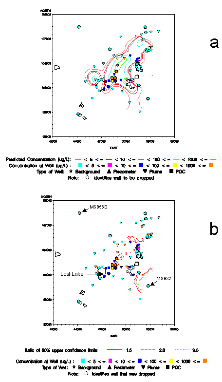
The well redundancy analyses are presented in Figures 1-3 below and show the kriging results for TCE for the Water Table, Upper Lost Lake, and Lower Lost Lake Aquifers, respectively. Panel a in each Figure shows the predicted TCE contours based on all well data from that aquifer. Panel b in each Figure shows the contour of the ratio of two upper 90% confidence limits (UCL90) of TCE concentration. The denominator is the UCL90 for the predicted concentration at that spatial location based on the data set containing all wells in the aquifer. The numerator is the UCL90 for the predicted concentration at that spatial location based on the well subset which does not contain the data for wells regarded as redundant, irrelevant, or unreliable. The latter wells were called "candidates" for exclusion.
In Fig. 1-3, the location of point-of compliance, background, or plume definition well types are represented by squares, stars, and hearts, respectively. The color of a symbol represents the TCE well concentration. The small circles around some of these figures represent the wells that are candidates for elimination. The black polygons represent seepage basins, rubble pits, and other landmarks.
The Water Table Aquifer
The TCE predictions in Figure 1a show concentrations contours at 5, 10, 100, and 1000 ug/L and was constructed by kriging over the set of all baseline wells. Well 56D in the Northwest portion of the map is far removed from the plume and not in its apparent path. It is not redundant (there is no other nearby well), but it has been placed on the candidate list because it is not relevant to plume monitoring. The TCE concentration in well 56D was measured at background levels. The major area of TCE contamination stretches from the northeast , southwest to Lost Lake.
A second dataset of kriged or predicted concentrations was generated by first excluding candidate wells. Figure 1b shows the resulting confidence ratio plot. A noticeable contour change occurs near well MSB 32 in the Southeast. This well was also recommended for deletion based on other considerations. Isoconcentration maps show that the well is side gradient to the plume and a potentiometric surface analysis indicated that the well is directly downgradient of a potentiometric high associated with an area of uncontaminated recharge. Because of its location, the well can only monitor that clean recharge and is therefore irrelevant.
Several smaller areas of change are observed in Figure 1b along the axis of relatively high concentrations between Lost Lake (polygon middle left) and the SRL Seepage Basins (polygons middle right). However, these are located in the central region of the plume, not affecting the capability of monitoring the direction and extent of any movement.
The Upper Lost Lake Aquifer
Figures 2a and 2b summarize the TCE results for the Upper Lost Lake Aquifer. Figure 2a is a baseline map of the predicted TCE concentration over the A/M Area using all well data. Again, a second kriged dataset was produced without the redundant well candidates. The confidence ratio plot (Fig. 2b) shows only two areas of contour change. In the Northwestern portion of the A/M Area a change occurs around wells AC 1A and AC 1B. The map’s uncertainty in this region is largely due to the fact that kriging ignores hydraulic gradient. AC 1A and AC 1B are safely side gradient of the plume, but the kriging program does not know this and shows contours with a side gradient bulge toward the deleted wells. However, the real users of the monitoring data know the flow direction and, hence, know that such a bulge is unlikely. So, in reality, wells MSB-30CC and SRW-2B offer sufficient control of the contours, and AC 1A and AC 1B can be deleted.
Figure 1. Kriging plots for TCE in Water Table aquifer in the
A/M area; a) predicted concentrations
before well data removal and b) the upper 90% confidence limit ratio to show
spatial
locations where predicted concentration changes occurred.
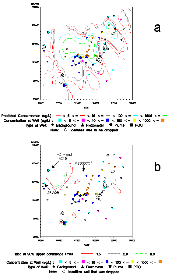
Figure 2. Kriging plots for TCE in Upper Lost Lake aquifer in
the A/M area; a) predicted concentrations
before well data removal and b) the upper 90% confidence limit ratio to show
spatial
locations where predicted concentration changes occurred.
The Lower Lost Lake Aquifer
Figures 3a and 3b depict the results for TCE in the Lower Lost Lake Aquifer. Figure 3a shows contour of the confidence ratio. There appears to be some contour change in the TCE concentration to the Northwest of the MSB 21 cluster and upgradient to the plume in the Northeast part of this well network.
The change contour near the MSB 21 cluster is the result of dropping MSB 21A with concentration 15 ug/L, while retaining the deeper well MSB 21B with a concentration of 240ug/L. This has increased the local prediction of TCE in the vicinity of cluster MSB 21. However, this change does not alter the ability to monitor the edge of the plume in the Northwest. Two change contours (2) appear in the Northeast. The elliptical change contour around only well MSB 82C is due to a local increase in the predicted TCE concentration. A second contour includes MSB 54C, MSB 83C, and MSB 84C. These changes result from a small local shift in the 5ug/L contour and should not bear on the ability to monitor the plume whose potentiometric surface slopes down toward the East.
Two additional confidence change contours lie to the South. One change contour covers MSB 87B and MSB 32B in the Southeast. These reflect the greater statistical uncertainty in the TCE predictions in the vicinity. However, MSB 19B provides sufficient protection to monitor the local extent of the plume. The other change contour encircles well MSB 79B. However, this region is near the plume boundary.
Analyte Reduction
The findings of Wells (1997) suggest that the groundwater monitoring program should be modified in the following ways. Semi-annual sampling for the inorganics in Section I of the Groundwater Protection Standards list (barium, cyanide, nickel, lead, and selenium) should only be performed at the POC and background wells. The "Inorganics" list in Section II should be shortened to include only nitrate, copper, zinc, chromium, mercury, uranium and cobalt. Annual monitoring for these constituents (with the exception of nitrate) should be continued only at the POC and background wells. Nitrate should be monitored at the POC wells, the background wells, and at well clusters MSB-17, MSB-18, and MSB-39.
Monitoring for radium should be discontinued. Monitoring for gross alpha and gross beta should continue only at the POC wells, the background wells and well clusters MSB-17, MSB-18 and MSB-39.
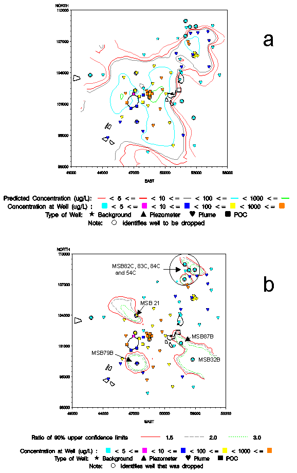
Figure 3. Kriging plots for TCE in Lower Lost Lake aquifer in
the A/M area; a) predicted concentrations before
well data removal and b) the upper 90% confidence limit ratio to show spatial
locations
where predicted concentration changes occurred.
Conclusions and Recommendations
We may conclude from this study that the integration of the elements of geochemistry, hydrogeology, geostatistics, and isoconcentration map analysis provides a technically sound basis for streamlining groundwater monitoring networks at SRS. The combined GME Team effort identified 16 more wells for elimination from the sampling schedule than had been identified previously through efforts in which the analytical elements were not integrated.
The following are the principal recommendations proposed and accepted by the regulator:
We believe further reductions in monitoring costs could accrue from the use of the Cost Effective Sampling (CES) technology. This technology has been recently developed and deployed by the Lawrence Livermore National Laboratory (Johnson et al. 1994) with some initial collaboration with SRTC statisticians. It is designed to review the change in constituent concentrations with time and establishes an algorithm for reducing the groundwater sampling frequency based on the statistically estimated rate of change. Low rates of change suggest an annual or even biannual sampling frequency, whereas high rates of change would substantiate a quarterly sampling frequency.
References
Appendix
Data Qualification
The water quality and analyte measurements for the A/M Well Network reside on the relational database, Geochemical Information Management System (GIMS). In addition to the water quality and analyte measurements, the database contains well location, depth, screening zones, installation and abandonment dates. The additional information is required for the geostatistical analyses.
Quering the GIMS database, over 400 analyte constituents were measured on samples from one or more of the A/M network wells over the period between 1Q1991 and 4Q1996. Many of the results were for constituents of very little interest, such as constituents with no results above detection in any of the wells for any of the quarters. The list of analyte constituents was narrowed to the four analytes of concern plus related analytes. The series of analytes initially plotted included: chloride, chlorobenzene, 1,1-dichloroethane, 1,1-dichloroethane, 1,2-dichloroethane, trans-1,2-dichloroethylene, 1,1-dichloroethylene, 1,2-dichloroethylene, gross alpha, nonvolatile beta, 1,1,1,2- tetrachloroethane, 1,1,2,2-tetrachcloroethane, tetrachloroethylene, 1,1,1-trichloroethane, 1,1,2-trichloroethane, trichloroethylene, nitrate-nitrate as nitrogen, and radium, total alpha emitting. Constituents were plotted over time separately by well in order to determine within well consistency and to visually examine differences between wells. The list of analytes was trimed to the four of concern before doing variograms and kriging.
For these four analytes, the results coded by the Environmental Monitoring Section (EMS) as unacceptable were rejected from further analysis. These results are coded with an "R" in the Result Qualifier Field in the GIMS database. The "R" means that the result should be rejected for almost all uses of the data. Acceptable results were examined for consistency of units over time, analytical laboratories, and analytical methods. The results were converted to converted to a common unit of measure: mg/L for Trichlorethylene and Tetrachoroethylene, pCi/L for Radium (total alpha emitting), and mg/L for Nitrate-Nitrite.
The remaining data were examined for large "less than detected" (LTD) results. Large LTD results generally exceed the largest measurement from a given well. Most of these large LTD results were due to large dilution factors, some as large as 106. To reduce the influence these large LTDs, we replaced them with the median reported LTD results for a given well and analyte from among all laboratories, analytical methods, and sampling dates. We also did not want to dilute the influence of the data above detection when the majority of the results within a quarter were above detection. To satisfy both criteria (1) minimize the influence of large "less than detected" results, and (2) not dilute true above detected results by averaging in replaced and smaller "less than detected" results, the following algorithm was used to identify and replace or omit large "less than detected" results.
First the median LTD reported result was determined for the four analytes over all wells, laboratories and methods. These were: 1.0 mg/L for Trichloroethylene and Tetrachcloroethylene, 0.05 mg/L for Nitrate-Nitrite, and 1.0 pCi/L for Radium (total alpha emitting).
Next, the percent of results above detection in each quarter and well was determined for each of the four analytes.
If at least 50% of the results were above detection, then all LTD results exceeding this median detection were omitted.
If more than 50% of the results were less than detection, then all LTD results exceeding the median detection were replaced with the median detected value.
This algorithm ensures that no undetected result enters into the analyses at a value greater than the median LTD reported result over all of the wells. Since the LTD results cannot exceed the results above detection in any well, LTD results will have minimal influence on wells within the plume, and will permit a sharper delineation between within and out of plume. After replacing or omitting LTD results, these remaining LTD results were divided by two.
The sample results, laboratory replicates, and the field and split sample duplicates within a quarter and well were averaged according to the following algorithm for each of the four analytes of concern.
Results within the same quarter, well, laboratory and analyzed by the same method were averaged first. If at least 50% of these measurements were above detection, then the method average was defined as above detection.
Next the method averages obtained in (1) were averaged over all possible methods used for that analyte by the laboratory within the same quarter for the same well. If at least 50% of the method averages were above detection, then the laboratory average was defined as above detection.
The laboratory averages found in (2) were averaged over all laboratories used
for the analyte, quarter and well to get a quarter average for each analyte,
well and quarter. If at least 50% of the laboratory averages were defined as
above detection, then the quarter averages were above detection.